First Steps
For a quick overview of key functionality you can also view this tutorial:
This tutorial will give you a high-level tour of kamu and show you how it works through examples.
We assume that you have already followed the installation steps and have kamu tool ready.
Not ready to install just yet?
Try kamu in this self-serve demo without needing to install anything.
Don’t forget to set up shell completions - they make using kamu a lot more fun!
The help command
When you execute kamu or kamu -h - the help message about all top-level commands will be displayed.
To get help on individual commands type:
kamu <command> -h
This will usually contain a detailed description of what command does along with usage examples.
Note that some command also have sub-commands, e.g. kamu repo {add,list,...}, same help pattern applies to those as well:
kamu repo add -h
Command help is also available online on CLI Reference page.
Ingesting data
Throughout this tutorial we will be using the Modified Zip Code Areas dataset from New York Open Data Portal.
Initializing the workspace
To work with kamu you first need a workspace. Workspace is where kamu will store important information about datasets and cached data. Let’s create one:
mkdir my_workspace
cd my_workspace
kamu init
A workspace is just a directory with .kamu folder where all sorts of data and metadata are stored. It behaves very similarly to .git directory version-controlled repositories.
As you’d expect the workspace is currently empty:
kamu list
Creating a dataset
One of the design principles of kamu is to know exactly where any piece of data came from. So it never blindly copies data around - instead we establish ownership and links to external sources.
We’ll get into the details of that later, but for now let’s create such link.

Datasets are created from dataset snapshots - special files that describe the desired state of the metadata upon creation.
We will use a DatasetSnapshot file from kamu-contrib repo that looks like this:
kind: DatasetSnapshot
version: 1
content:
  name: us.cityofnewyork.data.zipcode-boundaries
  kind: Root
  metadata:
    - kind: SetPollingSource
      fetch:
        kind: Url
        # Dataset home: https://data.cityofnewyork.us/Health/Modified-Zip-Code-Tabulation-Areas-MODZCTA-/pri4-ifjk
        url: https://data.cityofnewyork.us/api/geospatial/pri4-ifjk?date=20240115&accessType=DOWNLOAD&method=export&format=Shapefile
      read:
        kind: EsriShapefile
      merge:
        kind: Snapshot
        primaryKey:
          # Modified ZIP Code Tabulation Area (ZCTA)
          # See for explanation: https://nychealth.github.io/covid-maps/modzcta-geo/about.html
          - modzcta
You can either copy the above into a example.yaml file and run:
kamu add example.yaml
Or add it directly from URL like so:
kamu add https://raw.githubusercontent.com/kamu-data/kamu-contrib/master/us.cityofnewyork.data/zipcode-boundaries.yaml
Such YAML files are called manifests. First two lines specify that the file contains DatasetSnapshot object and then specify the version of the schema, for upgradeability:
kind: DatasetSnapshot
version: 1
content: ...
Next we give dataset a name and declare its kind:
name: us.cityofnewyork.data.zipcode-boundaries
kind: Root
Datasets that ingest external data in kamu are called Root datasets.
Next we have:
metadata:
  - kind: ...
    ...
  - kind: ...
    ...
This section contains one or many metadata events that can describe different aspects of a dataset, like:
- where data comes from
- its schema
- license
- relevant documentation
- query examples
- data quality checks
- and much more.
kamu new command - it outputs a well-annotated template that you can customize for your needs.Dataset Identity
During the dataset creation it is assigned a very special identifier.
You can see it by running:
kamu list -w
┌───────────────────────────────────────────────────────────────────────────────┬──────────────────────────────────────────┬─────┐
│                                      ID                                       │                   Name                   │ ... │
├───────────────────────────────────────────────────────────────────────────────┼──────────────────────────────────────────┼─────┤
│ did:odf:fed01057c94fb0378e3222704bb70a261d3ebeaa0d1b38c056a0bdd476360b8548db1 │ us.cityofnewyork.data.zipcode-boundaries │ ... │
└───────────────────────────────────────────────────────────────────────────────┴──────────────────────────────────────────┴─────┘
Or:
kamu log us.cityofnewyork.data.zipcode-boundaries
Block #0: ...
SystemTime: ...
Kind: Seed
DatasetKind: Root
DatasetID: did:odf:fed01057c94fb0378e3222704bb70a261d3ebeaa0d1b38c056a0bdd476360b8548db1
This is a globally unique identity which is based on a cryptographic key-pair that only you control.
Thus by creating an ODF dataset you get both:
- a way to uniquely identify it on the web
- and a way to prove ownership over it.
This will be extremely useful when we get to sharing data with others.
Fetching data
At this point our new dataset is still empty:
kamu list
┌──────────────────────────────────────────┬──────┬────────┬─────────┬──────┐
│                   Name                   │ Kind │ Pulled │ Records │ Size │
├──────────────────────────────────────────┼──────┼────────┼─────────┼──────┤
│ us.cityofnewyork.data.zipcode-boundaries │ Root │   -    │       - │    - │
└──────────────────────────────────────────┴──────┴────────┴─────────┴──────┘
But the SetPollingSource
event that we specified in the snapshot describes where from and how kamu can ingest external data.
Polling sources perform following steps:
fetch- downloading the data from some external source (e.g. HTTP/FTP)prepare(optional) - preparing raw binary data for ingestion (e.g. extracting an archive or converting between formats)read- reading the data into a structured form (e.g. from CSV or Parquet)preprocess(optional) - shaping the structured data with queries (e.g. to convert types into best suited form)merge- merging the new data from the source with the history of previously seen data
You can find more information about data sources and ingestion stages in this section.
Note that the data file we are ingesting is in ESRI Shapefile format, which is a widespread format for geo-spatial data, so we are using a special EsriShapefile reader.
To fetch data from the source run:
kamu pull --all
At this point the source data will be downloaded, decompressed, parsed into the structured form, preprocessed and saved locally.
kamu list
┌──────────────────────────────────────────┬──────┬───────────────┬─────────┬──────────┐
│                   Name                   │ Kind │    Pulled     │ Records │   Size   │
├──────────────────────────────────────────┼──────┼───────────────┼─────────┼──────────┤
│ us.cityofnewyork.data.zipcode-boundaries │ Root │ X seconds ago │     178 │ 1.87 MiB │
└──────────────────────────────────────────┴──────┴───────────────┴─────────┴──────────┘
Note that when you pull a dataset, only the new records that kamu hasn’t previously seen will be added. In fact kamu preserves the complete history of all data - this is what enables you to have stable references to data, lets you “time travel”, and establish from where and how certain data was obtained (provenance). We will discuss this in depth in further tutorials.
For now it suffices to say that all data is tracked by kamu in a series of blocks. The Committed new block X message you’ve seen during the pull tells us that the new data block was appended. You can inspect these blocks using log command:
$ kamu log us.cityofnewyork.data.zipcode-boundaries
Exploring data
Since you might not have worked with this dataset before you’d want to explore it first.
For this kamu provides many tools (from basic to advanced):
tailcommand- SQL shell
- Jupyter notebooks integration
- Web UI
Tail command
To quickly preview few last events of any dataset use tail command:
$ kamu tail us.cityofnewyork.data.zipcode-boundaries
SQL shell
SQL is the lingua franca of the data science and kamu uses it extensively. So naturally it provides you a simple way to run ad-hoc queries on data.
Following command will drop you into the SQL shell:
kamu sql
By default this command uses the Apache Datafusion engine, so its powerful SQL is now available to you.
All datasets in your workspace should be available to you as tables:
show tables;
You can use describe to inspect the dataset schema:
describe "us.cityofnewyork.data.zipcode-boundaries";
And of course you can run queries against any dataset:
select
  *
from "us.cityofnewyork.data.zipcode-boundaries"
order by pop_est desc
limit 5;
Use Ctrl+D to exit the SQL shell.
SQL is a widely supported language, so kamu can be used in conjunction with many other tools that support it, such as Tableau and Power BI. See integrations for details.
The kamu sql is a very powerful command that you can use both interactively or for scripting. We encourage you to explore more of its options through kamu sql --help.
Notebooks
Kamu lets you access the power of multiple data engines through a convenient interface of Jupyter Notebooks.
Get started by running:
kamu notebook -e MAPBOX_ACCESS_TOKEN=<your mapbox token>
kamu to pass the MapBox access token as MAPBOX_ACCESS_TOKEN environment variable into Jupyter, which we will use for plotting. You can get the token for free or skip this step and simply run kamu notebook.Executing this should open your default browser with a Jupyter running in it.
From here let’s create a notebook and start it by loading kamu extension:
%load_ext kamu
We then need to create a connection:
import kamu
con = kamu.connect()
The kamu Python library will automatically connect to your local workspace node.
After this the import_dataset command becomes available and we can load the dataset and alias it by doing:
You can now query the datasets using the connection:
con.query("select * from 'us.cityofnewyork.data.zipcode-boundaries' limit 3")
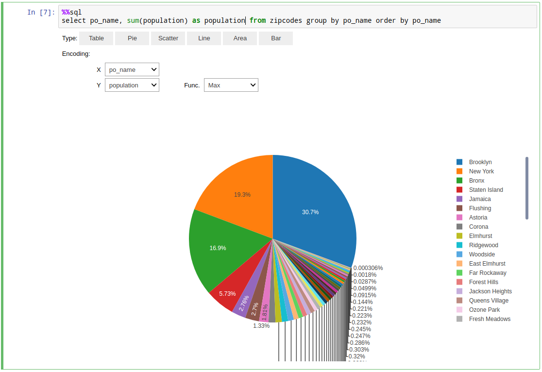
Or, more conveniently, using the %%sql cell magic:
%%sql
select * from 'us.cityofnewyork.data.zipcode-boundaries' limit 3
The queries return regular Pandas dataframe.
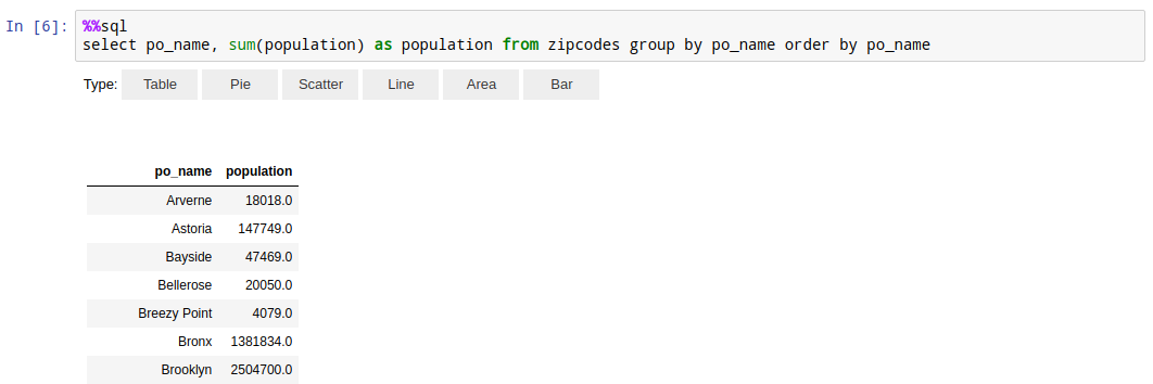
Thanks to the autovizwidget library you also get some simple instant visualizations for results of your queries.
To assign the result of %%sql cell to a variable use:
%%sql -o population_density
select ...
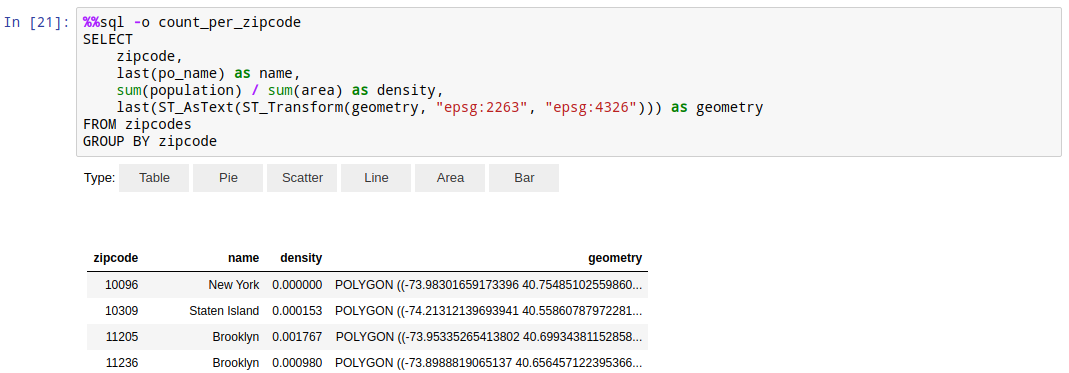
You can use any of your favorite libraries to further process and visualize it:
Example of visualizing population density data as a choropleth chart using mapboxgl library:
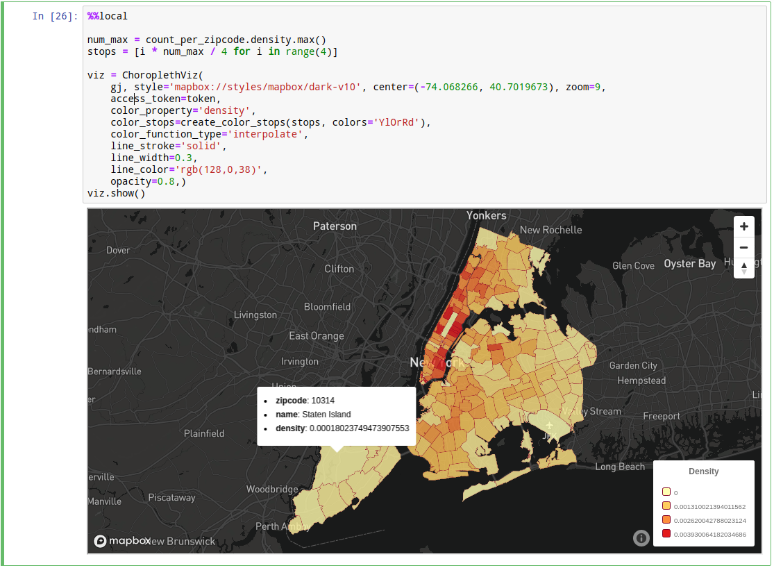
You can find this as well as many other notebooks in kamu-contrib repo.
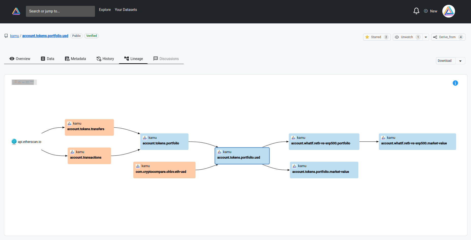
Web UI
All the above and more is also available to you via embedded Web UI which you can launch by running:
kamu ui
Web UI is especially useful once you start developing complex stream processing pipelines, to explore them more visually:
Conclusion
We hope this quick overview inspires you to give kamu a try!
Don’t get distracted by the pretty notebooks and UIs though - we covered only the tip of the iceberg. The true power of kamu lies in how it manages data, letting you to reliably track it, transform it, and share results with your peers in an easily reproducible an verifiable way.
Please continue to the self-serve demo for some hands-on walkthroughs and tutorials, and check out our other learning materials.