Stock Market Trading

Topics covered:

• Temporal aggregations (cumulative sum)
• Temporal table joins
• Watermarks

Summary

Stock market data analysis is one of the problems where time dimension plays a crucial importance and cannot be left out. This example shows how kamu and streaming SQL can be used to build your personal trading performance dashboard which is more powerful than what most trading platforms provide. You will learn how to perform aggregations and join temporal stream and the role of watermarks in this process.

Steps

Getting Started

To follow this example checkout kamu-cli repository and navigate into examples/trading sub-directory.

Create a temporary kamu workspace in that folder using:

kamu init

You can either follow the example steps below or fast-track through it by running:

# Add all dataset manifests found in the current directory
kamu add --recursive .
kamu pull --all

Root Datasets

We will be using two root datasets:

• com.yahoo.finance.tickers.daily - contains daily price summaries (candles) of several major tickers.
• my.trading.transactions - contains a log of transaction from a fake trading account similar to what you’d get in data export from your trading platform.

Both datasets are sourcing their data from files located in data/ sub-directory. Once comfortable with this example you can explore sourcing ticker data from external financial APIs (e.g. as name suggests from finance.yahoo.com) and using your own trading transaction history.

Let’s add the root datasets and ingest data:

kamu add com.yahoo.finance.tickers.daily.yaml my.trading.transactions.yaml
kamu pull --all

You can verify the result using tail command or the SQL shell:

kamu sql

0: kamu> select * from `com.yahoo.finance.tickers.daily` limit 5;
+-------------+------------+---------+------------+-----------+-----------+-----------+-----------+-----------------+
| system_time | event_time | symbol  | close_adj  |   close   |   high    |    low    |   open    |     volume      |
+-------------+------------+---------+------------+-----------+-----------+-----------+-----------+-----------------+
|     ...     | 2016-01-04 | IPO     | 19.8662    | 20.2800   | 20.6000   | 20.1700   | 20.6000   | 3800.0000       |
|     ...     | 2016-01-04 | SPY     | 183.2916   | 201.0200  | 201.0300  | 198.5900  | 200.4900  | 222353500.0000  |
|     ...     | 2016-01-05 | SPY     | 183.6017   | 201.3600  | 201.9000  | 200.0500  | 201.4000  | 110845800.0000  |
|     ...     | 2016-01-05 | IPO     | 19.8173    | 20.2300   | 20.2800   | 20.2000   | 20.2800   | 4000.0000       |
|     ...     | 2016-01-06 | IPO     | 19.4156    | 19.8200   | 20.0600   | 19.8200   | 19.9700   | 2600.0000       |
+-------------+------------+---------+------------+-----------+-----------+-----------+-----------+-----------------+

Remember that after adding a dataset from a yaml file - kamu creates an internal representation of it in the workspace .kamu directory, so if you want to make any changes to the dataset you will need to re-add the dataset again after changing the yaml file.

kamu delete com.yahoo.finance.tickers.daily
# ... Make changes to the yaml file ...
kamu add com.yahoo.finance.tickers.daily.yaml

# Or alternatively
kamu add --replace com.yahoo.finance.tickers.daily.yaml

Deriving current holdings from the transaction log

Our first goal will be to visualize the market value of our account. The account’s market value can be estimated by multiplying the number of stocks held by their last known ticker price. Of course we aren’t as interested in current market value as in dynamics of how it was changing over time, so we’d want to produce a stream of events telling us the estimated market value at different points in time.

If you look at the my.trading.transactions dataset it essentially contains deltas: how many stocks were bought/sold in each transaction, and the settlement amounts going in/out of our cache account. Our first step, therefore, should be obtaining a dataset that can tell us how many stocks in total (per symbol) we own. This can be easily achieved by calculating a running cumulative sum over stock quantities bought and sold.

Since this data might be something we can reuse in other calculations - let’s create a dedicated derivative dataset for it.

The following listing shows the use of Flink engine and the SQL window functions for enriching all transaction events with cumulative sums of stock quantities and cash put into buying them:

kind: DatasetSnapshot
version: 1
content:
  name: my.trading.holdings
  kind: Derivative
  metadata:
    - kind: SetTransform
      inputs:
        - datasetRef: my.trading.transactions
      transform:
        kind: Sql
        engine: flink
        query: |
          SELECT
            event_time,
            symbol,
            quantity,
            price,
            settlement,
            sum(quantity) over(partition by symbol order by event_time rows unbounded preceding) as cum_quantity,
            sum(settlement) over(partition by symbol order by event_time rows unbounded preceding) as cum_balance
          FROM `my.trading.transactions`          

Let’s create this dataset:

kamu add my.trading.holdings.yaml
kamu pull my.trading.holdings

The result should look something like:

kamu tail my.trading.holdings

+-------------+------------+---------+-----------+-----------+-------------+---------------+--------------+
| system_time | event_time | symbol  | quantity  |   price   | settlement  | cum_quantity  | cum_balance  |
+-------------+------------+---------+-----------+-----------+-------------+---------------+--------------+
|     ...     | 2016-01-04 | SPY     | 1         | 201.0200  | -201.0200   | 1             | -201.0200    |
|     ...     | 2016-02-01 | SPY     | 1         | 193.6500  | -193.6500   | 2             | -394.6700    |
|     ...     | 2016-03-01 | SPY     | 1         | 198.1100  | -198.1100   | 3             | -592.7800    |
|     ...     | 2016-04-01 | SPY     | 1         | 206.9200  | -206.9200   | 4             | -799.7000    |
|     ...     | 2016-05-02 | SPY     | 1         | 207.9700  | -207.9700   | 5             | -1007.6700   |
+-------------+------------+---------+-----------+-----------+-------------+---------------+--------------+

Calculating current market value of held positions

Now that we have enriched our transaction data with a running total of holding calculating market value should be a matter of joining these value with the ticker price data.

In the non-temporal world we could solve this problem as:

holdings:              tickers:
+--------+----------+  +--------+----------+
| symbol | quantity |  | symbol | price    |
+--------+----------+  +--------+----------+
| SPY    | 50       |  | SPY    | 257.9700 |
+--------+----------+  +--------+----------+

SELECT
    h.symbol,
    h.quantity,
    h.price as price_unit,
    h.quantity * h.price as price_total
FROM tickers as t
LEFT JOIN holdings as h ON t.symbol = h.symbol

In our case, however, we are joining two streams of events, which might be new to many people.

Consider, for example, the following event in tickers:

+-------------+------------+---------+------------+-----------+-----------+-----------+-----------+-----------------+
| system_time | event_time | symbol  | close_adj  |   close   |   high    |    low    |   open    |     volume      |
+-------------+------------+---------+------------+-----------+-----------+-----------+-----------+-----------------+
|     ...     | 2016-01-06 | SPY     | 181.2856   | 198.8200  | 200.0599  | 197.600   | 198.3399  | 152112600.0000  |
+-------------+------------+---------+------------+-----------+-----------+-----------+-----------+-----------------+

When we join it with holdings data we would like it to be joined with the holdings event that directly precedes it in the event time space - current price joined to the value of portfolio at that time. In our example it would be:

+-------------+------------+---------+-----------+-----------+-------------+---------------+--------------+
| system_time | event_time | symbol  | quantity  |   price   | settlement  | cum_quantity  | cum_balance  |
+-------------+------------+---------+-----------+-----------+-------------+---------------+--------------+
|     ...     | 2016-01-04 | SPY     | 1         | 201.0200  | -201.0200   | 1             | -201.0200    |
+-------------+------------+---------+-----------+-----------+-------------+---------------+--------------+

There are two ways to achieve this. We could use stream-to-stream joins and describe the tolerance intervals (how far two events can be apart from each other in time) and the “precedes” condition in our join statement. While stream-to-stream joins have valuable applications using them in this case would be too cumbersome. Instead, we can use the temporal table joins.

Temporal table joins (see this great explanation in Apache Flink’s blog) take one of the streams and represent it as a three-dimensional table. You can think of it as holdings table from the non-temporal example above that has a third “depth” axis which is event_time. When joining to such a table you need to pass in the time argument to tell the join which version of the table to consider.

Let’s have a look at the my.trading.holdings.market-value dataset:

kind: DatasetSnapshot
version: 1
content:
  name: my.trading.holdings.market-value
  kind: Derivative
  metadata:
    - kind: SetTransform
      inputs:
        - datasetRef: com.yahoo.finance.tickers.daily
        - datasetRef: my.trading.holdings
      transform:
        kind: Sql
        engine: flink
        temporalTables:
          - name: my.trading.holdings
            primaryKey:
              - symbol
        query: |
          SELECT
            tickers.`event_time`,
            holdings.`symbol`,
            holdings.`cum_quantity`,
            holdings.`quantity` as `quantity`,
            tickers.`close_adj` * holdings.`cum_quantity` as `market_value`
          FROM `com.yahoo.finance.tickers.daily` as tickers
          JOIN `my.trading.holdings` FOR SYSTEM_TIME AS OF tickers.`event_time` AS holdings
          ON tickers.`symbol` = holdings.`symbol`          

Using temporalTables section we instruct the Flink engine to use my.trading.holdings event stream to create a virtual temporal table of the same name.

Here’s how this three-dimensional table would look like when sliced at different points in time:

my.trading.holdings:

@ 2016-01-04
+---------+---+---------------+--------------+
| symbol  |...| cum_quantity  | cum_balance  |
+---------+---+---------------+--------------+
| SPY     |   | 1             | -201.0200    |
+---------+---+---------------+--------------+

@ 2016-02-01
+---------+---+---------------+--------------+
| symbol  |...| cum_quantity  | cum_balance  |
+---------+---+---------------+--------------+
| SPY     |   | 2             | -394.6700    |
+---------+---+---------------+--------------+

@ 2016-03-01
+---------+---+---------------+--------------+
| symbol  |...| cum_quantity  | cum_balance  |
+---------+---+---------------+--------------+
| SPY     |   | 3             | -592.7800    |
+---------+---+---------------+--------------+

It basically remembers the last observed value of every column grouped by the provided primaryKey (symbol in our case).

The JOIN my.trading.holdings FOR SYSTEM_TIME AS OF tickers.event_time part can be interpreted as us taking every ticker event from tickers, indexing the temporal table my.trading.holdings at this event’s event_time and then joining the same event with the resulting (now ordinary two-dimensional) table.

With theory out of the way, time to give this a try:

kamu add my.trading.holdings.market-value.yaml
kamu pull my.trading.holdings.market-value

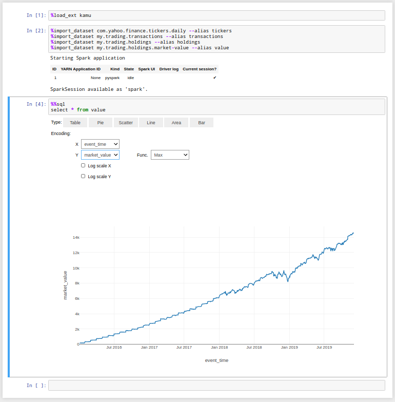
To view the results you can use the provided trading.ipynb notebook and see the actual graph:

kamu notebook

The role of watermarks

If you look closely at the previous graph you will notice that the last event there is dated 2019-12-02. This might be surprising because even though our account has stopped actively trading on that date, the ticker data still keeps coming, so we should be seeing the market value change over the course of 2020 and onwards…

Congratulations, you have just stumbled onto one of the most important features that distinguishes stream processing queries from batch processing!

When joining two streams kamu and its engines can’t make any guesses about how complete the data in your dataset is. The streams you are joining can have vastly different intervals with which data is added. Ticker data might be added daily, while you, as the owner of transactions dataset, might be exporting your trading data semi-regularly, once in a month or two. Therefore when the transaction data stops coming on Dec 2 2019 it means that kamu can’t tell whether you are not actively trading any more or you simply forgot to import the recent transaction history. It therefore pauses the processing until this ambiguity is resolved (effectively by starting to buffer the ticker data).

The property behind this mechanism is called watermark. The watermark is a simple timestamp T that tells that with a high probability all events before T have already been ingested into the system. You can take a look at your dataset’s watermarks using the log command:

kamu log my.trading.transactions

Block #3: f16201cfd3c1822add90232665e78e94092d027ec87f93dd7410fc59104262cfbf378
SystemTime: 2024-01-16T00:42:57.722238098Z
Kind: AddData
NewData:
  NumRecords: 48
  Size: 3564
  ...
NewSourceState: ...
NewWatermark: 2019-12-02T00:00:00Z

There are two ways to resolve the “no data vs. stale data” ambiguity and advance the watermark:

• Adding data - by default kamu advances the watermark to the latest observed event time of the stream. This is not always what you want - if your data often arrives late and out of order it might be wise to delay the watermark to maximize the chances that further processing will not have to deal with late data.
• Advancing watermark manually - doing this tells kamu that we don’t expect any data prior to some time T to arrive any more.

Using manual watermarks

Let’s put this into practice and tell kamu that transaction data is complete as of 2020-09-01:

kamu pull my.trading.transactions --set-watermark 2020-09-01T00:00:00Z

As you can see, this commits a watermark-only metadata block:

kamu log my.trading.transactions

Block #4: f1620c4951a20fccd02e9125497b7c1e032f4d22de8c71b1cade3824c15bf61258161
SystemTime: 2024-01-16T00:45:22.998784847Z
Kind: AddData
PrevOffset: 47
NewWatermark: 2020-09-01T00:00:00Z

You can also use the short-hand forms like:

kamu pull my.trading.transactions --set-watermark '1 month ago'

If we now pull the market value dataset we will see new data emitted:

kamu pull my.trading.holdings.market-value --recursive

You can now reload the notebook and see that the graph extends to our watermark date.