Housing Prices

Topics covered:

• GIS functions
• Spatial joins
• Notebooks

Summary

Geospatial data is so widespread that no data science software would be complete without ability to manipulate it efficiently. In this example we will take a look how GIS data can be used in kamu using Apache Spark engine that comes with Apache Sedona extension.

Steps

Getting Started

To follow this example checkout kamu-cli repository and navigate into examples/housing_prices sub-directory.

Root Datasets

We will be using following root datasets:

• ca.vancouver.opendata.property.tax-reports - contains property assessment reports from the city of Vancouver
• ca.vancouver.opendata.property.parcel-polygons - contains geographical outlines of properties
• ca.vancouver.opendata.property.block-outlines - contains geographical block outlines
• ca.vancouver.opendata.property.local-area-boundaries - contains outlines and names of Vancouver’s districts

For geospatial data kamu supports several input formats including ESRI Shapefile and GeoJson. Take a look at dataset definitions to understand how data is being ingested.

Quite often when ingesting GIS data you will need to deal with different projections. Example below shows how you can use a pre-processing step to convert data into another projection:

preprocess:
  kind: Sql
  engine: spark
  query: |
    SELECT
      ST_Transform(geometry, "epsg:3157", "epsg:4326") as geometry
    FROM input    

Note: epsg:4326 is one of the more commonly used projections which is expected by many visualization tools.

The ST_Transform function here comes from Apache Sedona extension for the Apache Spark engine for working with GIS data. We will be relying on many of its function throughout this example.

Lets add all these datasets to our workspace and ingest them:

# Create a kamu workspace in the example folder
kamu init

# Add all dataset manifests found in the current directory
kamu add --recursive .
kamu pull --all

# Alternatively: Pull datasets in ODF format from Kamu's repository
./init-s3.sh

This may take 10+ minutes as the tax report dataset is quite large. You can leave the ingest running and move on to the next step meanwhile.

Creating MapBox Account

For visualizing the GIS data we will be using the awesome Mapbox SDK. To follow the example you will need to create a free account and get your own access token. The token should look something like pk.eyJ...T6Q.

Visualizing Housing Prices

Once you have downloaded all datasets we can start with a simple notebook to get a feel for GIS visualization.

Start the notebook server and pass it your Mapbox token via environment variable:

kamu notebook -e MAPBOX_ACCESS_TOKEN=<your mapbox token>

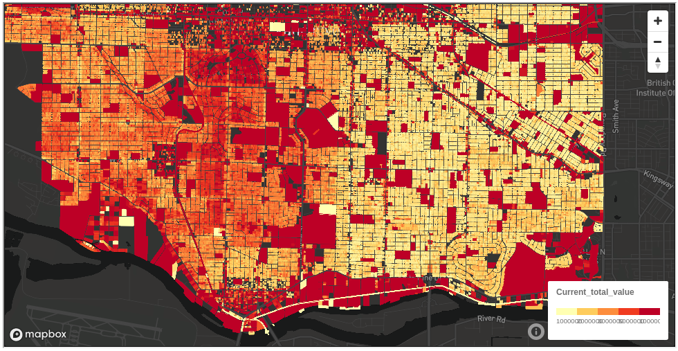
Now you can open the heatmap.ipynb and run through it executing each step. The notebook is pretty straightforward - it joins together the tax-reports dataset containing assessment values with parcel-polygons dataset containing land geometries in order to produce a heatmap.

%%sql
CREATE OR REPLACE TEMP VIEW lot_tax AS (
  SELECT
      t.*,
      l.geometry
  FROM lots as l
  JOIN tax as t
  ON l.tax_coord = t.land_coordinate
  WHERE
      t.legal_type = 'LAND'
      AND t.tax_assessment_year = 2019
      AND t.current_land_value is not null
)

It then pulls the result from Spark into the notebook itself using this query:

%%sql -o df -n 100000
SELECT
    land_coordinate,
    ST_AsGeoJSON(geometry) as geometry,
    current_land_value + current_improvement_value as current_total_value
FROM lot_tax

The -n 100000 parameter here overrides the default limit on the dataframe size, while ST_AsGeoJSON(geometry) also converts the internal binary geometry type into the GeoJson format. We later use custom-written df_to_geojson to combine individual geometries into GeoJson’s FeatureCollection objectm understood by the mapboxgl library.

We can then use the resulting GeoJson data and render the heatmap using the mapboxgl-jupyter library which comes pre-installed with kamu’s notebook server image.

Spatial Joins

Let’s take a look how datasets can be joined using the geometries. The local-area-boundaries contains the names of the Vancouver’s neighbourhoods along with their geographical boundaries. We also have the block-outlines dataset containing boundaries of individual blocks, but there’s an issue - there is no identifier that would link a block to a specific neighbourhood. For us to associate a block with the neighbourhood we have to see if block’s boundaries are contained or intersect the boundaries of some neighbourhood. Apache Sedona used by kamu optimizes such spatial joins.

You can open up the spatial_join.ipynb notebook and run through it step by step. The most important part ther is the join itself:

CREATE OR REPLACE TEMP VIEW blocks_by_hood AS (
    SELECT h.name, b.geometry
    FROM blocks as b
    INNER JOIN hoods as h
    ON ST_Intersects(b.geometry, h.geometry)
)

The rest of the visualization steps should be familiar to you from the previous example.

As an exercise - see if you can replace the median_value column that we have populated with RAND() for every block with an actual median property price. Just like before, there is unfortunately no identifier that would tie the property to a specific block, but see if Sedona can handle a massive spatial join between blocks and individual property outlines.